Exciting news about parameters

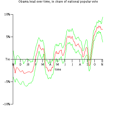
Possibly the most important parameters in my methodology are the assumed volatility of public opinion and the formula for assumed correlations between states. For most of this year, I've been assuming that one standard deviation of one-day national public opinion change is 0.2% and correlations of 95%+ between states, numbers that I chose because they looked roughly right from the data I saw, and because they gave results that made sense to me. However, ever since I saw the graph on this post from 538, I've worried that the volatility assumption was somewhat too low. So, over the weekend, I came up with a reasonable way to assess parameters from available 2008 data. More on that below the fold.

The main point is, now that I have a better grasp of the parameters I'm using, I have much greater confidence about my analysis than I ever have before. Additionally, I adjusted my estimates of voter turnout by scaling the 2004 turnout up by the increase in a state's voting-eligible population.

(By the way, I now believe that the graph I linked to above is somewhat misleading. I was only 10 in 1992, but as I recall Ross Perot's share of the vote plummeted after he bizarrely left and re-entered the race. I believe this is what produces the high-error dots early in the 1992 campaign.)

The key insight for setting parameters is this. Let's say I run the algorithm to generate estimates for each day during the campaign. If the algorithm's parameters are set correctly, then the polling data should tend to equal the estimate plus/minus a predictable error range. If the polling data are skewed to one side of the estimates, if the polling data match the estimates more closely than expected, or if the polling data match the estimates less closely than expected, then the parameters are bad.

For each date during the campaign and for each geographical unit, my algorithm produces (among other data) an estimate of the Obama-McCain difference in public opinion and the uncertainty of that estimate. Now suppose A is the uncertainty of my estimate on the polling date (i.e., one standard deviation of the difference between my estimate and the platonic truth), B is the poll's sample error, and C is the poll's non-sample error (which I assume is 2%). These are the three components of the difference between my estimate of the Obama-McCain difference (E) and the poll's estimate of the Obama-McCain difference (P), and it's reasonable to assume that these sources are independent. Then I expect the poll's estimate of the Obama-McCain difference to be normally distributed with an expected value of my estimate of the Obama-McCain difference and a standard deviation of sqrt(A^2+B^2+C^2).

In other words, if I list out the statistic (P-E)/sqrt(A^2+B^2+C^2) for each poll, I expect the list to have a standard normal distribution. To measure how close it is to a standard normal distribution, I first measure the mean (m) and standard deviation (s) of this statistic. Then, I evaluate the integral of [pdf(0,1)-pdf(m,s)]^2, where pdf(x,y) is the probability density function of the normal distribution with mean x and standard deviation y. Clearly, lower values of this integral signal a better distribution of polls around my estimates, which signals better parameters.

So far, the best parameters I've found are a daily national volatility of 0.245% and a correlation between each pair of states of 92%.

Read more (maybe)!